Mixed-Effect Modeling using MATLAB

Linear Mixed-Effect (LME) Models are generalizations of linear regression models for data that is collected and summarized in groups. Linear Mixed- Effects models offer a flexible framework for analyzing grouped data while accounting for the within-group correlation often present in such data.

This example illustrates how to fit basic hierarchical or multilevel LME models.

Copyright (c) 2014, MathWorks, Inc.

Contents

Description of the Data

This dataset consists of annual observations of 48 Continental U.S. States, over the period 1970–86 (17 years). This data set was provided by Munnell (1990)

Reference:

Load Data

clear, clc, close all
loadPublicData

If you don't have the data. You can download the Zip file from here.

Preprocess Data

Convert STATE, YR and REGION to categorical, In Matlab 2021, its appear as a default that you will get it as a categorical 

publicdata.STATE = categorical(publicdata.STATE);

% Compute log(GDP)

publicdata.log_GDP = log(publicdata.GDP);
publicdata.GDP = [];

Fit a linear model and visualize the Gross State Product by region

The formula is 

\( \epsilon_i \sim N(0,\sigma^2) \)

The data is collected between the years 1970 and 1986 for each state. When fitting a linear model, the intercept represents a GDP at YEAR 0. This may lead to an unusually low intercept, compensated by a large slope. This results in a high negative correlation between the estimates of the slopes and their corresponding intercept estimate. We can remove this correlation by centring the data.

Why do we need to centre the data? 

publicdata.YRcentered = publicdata.YR - mean(unique(publicdata.YR));
lm = fitlm(publicdata,'log_GDP ~ 1 + YRcentered');

Visualize data and fitted model

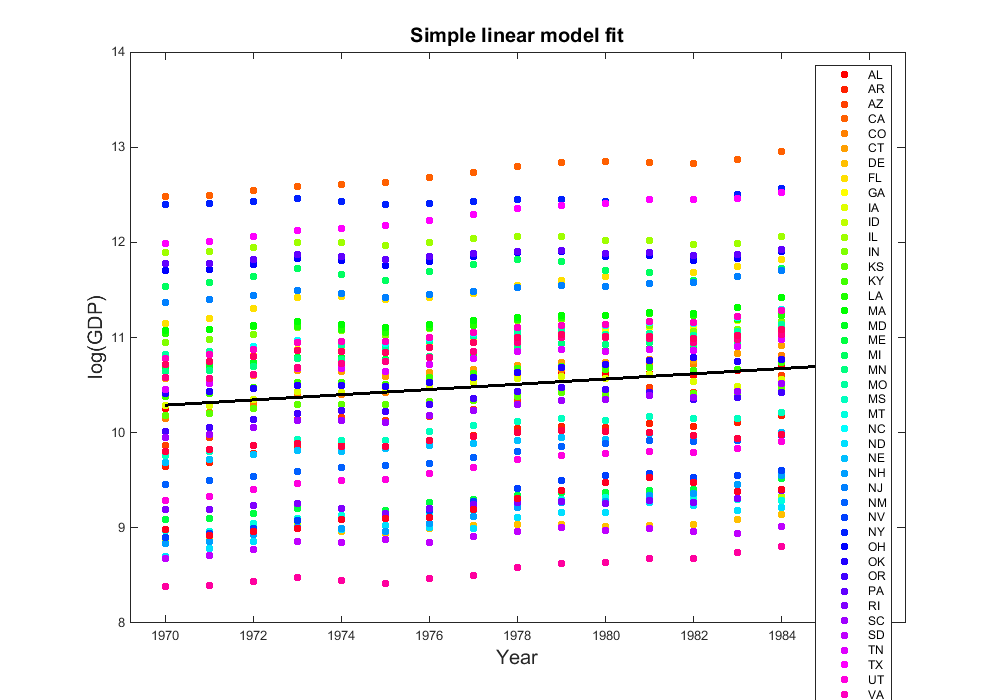
figure,
gscatter(publicdata.YR,publicdata.log_GDP,publicdata.STATE,[],'.',20);
hold on
plot(publicdata.YR,predict(lm),'k-','LineWidth',2)
title('Simple linear model fit','FontSize',15)
xlabel('Year','FontSize',15), ylabel('log(GDP)','FontSize',15)

From the figure, it is clear that fitting a simple linear regression model that ignores state (or region) specific information is not sufficient to fully specify the relationship between log_GDP and YR. All the unmodelled group-specific (contextual) information ends up pooled into a single error term. This means we ignore any error correlation within a group violating assumptions of linear regression and leading to biased standard errors.

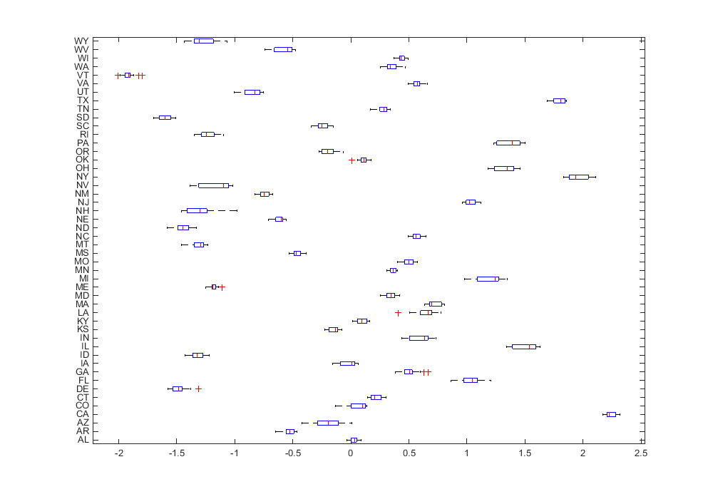
figure,
xlabel('OLS Residuals')
boxplot(lm.Residuals.Raw,publicdata.STATE,'orientation','horizontal')

The boxplot of OLS residuals by STATE shows that the within state residuals are either all positive or all negative and are not centred at 0. This violates the fundamental assumption of OLS and the resulting inference may not be valid.

Fit separate linear models per group and visualize intervals of parameters

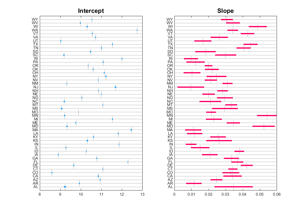
figure,
plotIntervals(publicdata,'log_GDP ~ 1 + YRcentered','STATE')

The individual confidence intervals give us a clear indication that a random effect is needed to account for the state to state variability in the intercept and slope since the confidence intervals don't overlap.

Fit a single linear model with dummy variables for each state

One way to go about incorporating group-specific effect using only fixed-effects is to introduce dummy variables for STATE and the interaction between STATE and YEAR as follows

lm_group = fitlm(publicdata,'log_GDP ~ 1 + YRcentered + STATE + YRcentered:STATE');

% Display the number of predictors and number of estimated coefficients.
disp(' ')
disp(['Number of Variables:', num2str(lm_group.NumPredictors)])
disp(['Number of Estimated Coefficients:', ...
    num2str(lm_group.NumEstimatedCoefficients)])

 
Number of Variables:2
Number of Estimated Coefficients:96

From the figure, it appears that this is a much better model than the earlier fit. It is only ideal when there are fewer levels in STATE and a lot of observations. There are several disadvantages to this approach. Even though the fixed-effects model accounts for the STATE effect, it does not provide a useful representation of the data since it only models the specific samples in the data which does not generalize to the population. Secondly, the number of free parameters in the model increases linearly with the number of levels in STATE and this results in a loss in degrees of freedom. This can be a problem when dealing with smaller sets of observations.

Fit a random intercept model

Let us explore a mixed-effect model where we allow the intercept to vary randomly for each group, in this case for each state. We have a fixed-effect for intercept and YRcentered

\( log\_GDP_{ij} = \beta_{00} + \beta_1 YR_{ij} + b_{0j} + \epsilon_{ij}\)

\(b_{0j} \sim N(0,\sigma_{b}^2) \)

\(\epsilon_{ij} \sim N(0,\sigma^2)\)

clc
lme_intercept = fitlme(publicdata,'log_GDP ~ 1 + YRcentered + (1|STATE)');

The standard deviation of the state random-effects term, do not include 0 (Lower:0.82594, Upper:1.2324), which indicates that the random-effects term is significant.

Fit a random intercept and slope model

(Latex)

\( log\_GDP_{ij} = \beta_{00} + \beta_{10} YR_{ij} + b_{0j} + b_{1j} YR_{ij} + \epsilon_{ij} \)

\( b = \left(\begin{array}{c} b_{0j}\\ b_{1j} \end{array}\right) \sim N(0,\Sigma) = N \left(0,\left(\begin{array}{cc} \sigma_{1}^2 & \sigma_{12}^2\\ \sigma_{12}^2 & \sigma_{2} \end{array}\right)\right) \)

\( \epsilon_{ij} \sim N(0,\sigma^2) \)

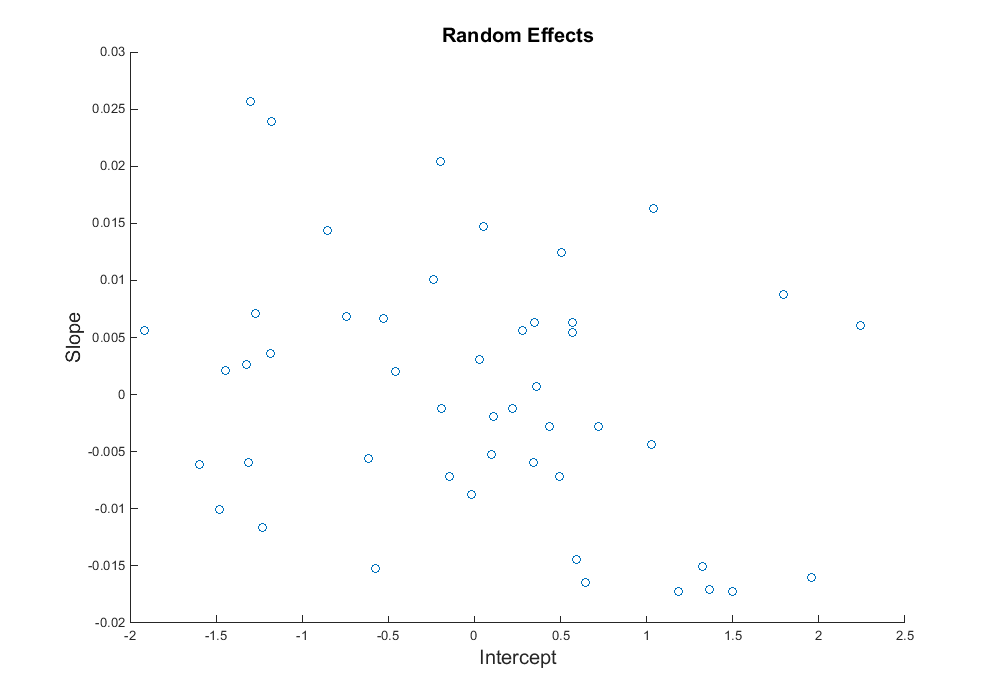
clc
lme_intercept_slope = fitlme(publicdata,...
    'log_GDP ~ 1 + YRcentered + (1+YRcentered|STATE)');

[~,~,rEffects] = randomEffects(lme_intercept_slope);

figure,
scatter(rEffects.Estimate(1:2:end),rEffects.Estimate(2:2:end))
title('Random Effects','FontSize',15)
xlabel('Intercept','FontSize',15)
ylabel('Slope','FontSize',15)
% The estimated column in the random-effects table shows the estimated best
% linear unbiased predictor (BLUP) vector of random effects.

Compare random slope and intercept models using Likelihood Ratio Test

A Likelihood Ratio Test (LRT) statistic can be used to determine if the more complex model is significantly better than the simpler model. Here we are comparing a random intercept model with a random slope and intercept model to determine the significance of introducing random-effect for slope.

compare(lme_intercept, lme_intercept_slope, 'CheckNesting',true)

ans = 


    THEORETICAL LIKELIHOOD RATIO TEST

    Model                  DF    AIC        BIC        LogLik    LRStat
    lme_intercept          4     -1550.5    -1531.7    779.24          
    lme_intercept_slope    6     -2085.4    -2057.2    1048.7    538.94


    deltaDF    pValue
                     
    2          0     

The small p-Value indicates that the second model which accounts for the possible correlation between the random effects is significantly better than first model. The flag 'CheckNesting' attempts to check that the first model is nested in the second model.

Fit Mixed-Effect models using matrix notation

(Latex)

\( y = X\beta + Zb + \epsilon \)

If you cannot easily describe your model using a formula, you can create design matrices to define the fixed and random effects, and then call fitlmematrix ;

y = X*beta + Z*b + e

We can reproduce the results for the model that had random intercept and slope, with the possible correlation between them

% Response (Dependent Variable)
y = publicdata.log_GDP;

% Fixed Effects Design Matrix
X = [ones(height(publicdata),1), publicdata.YRcentered];
% Random Effects Design Matrix
Z = [ones(height(publicdata),1), publicdata.YRcentered];

% Grouping Variable
G = publicdata.STATE;

% The random-effects design matrix can optionally include the dummy coded
% variable for the group. If however group 'G' is provided, fitlmematrix
% automatically does this for you.

% Fit the model
lme_matrix = fitlmematrix(X,y,Z,G,'CovariancePattern','Diagonal');

Forecast state GDP

states = {'IL','NJ','MA','CT','UT','NV','VT','WY'};
unbalancedStates = {'IL','CT','WY'};
missingYears = 1970:1983;
compareForecasts(publicdata, states, unbalancedStates, missingYears)

The figure shows a comparison of GDP forecasts using the two approaches. Solid circles indicate observations that were used to fit the model and empty circles indicate observations that were excluded from the model but shown for visual validation of the forecast.

The first plot shows the forecast of a Fixed-Effects model which incorporates group-specific effects using dummy variables for STATE and STATE:YEAR. The second plot shows the forecast of an LME model with a random slope and intercepts model. The confidence intervals for the forecast show that the LME model gives you a much more confident forecast even in the presence of missing data.

A closer look at WY shows that due to the small number of observations available, the Fixed-Effects model shows a decreasing GDP forecast over time. LME model on the other hand captures the overall trend of the data as a whole and forecasts an increasing GDP which agrees with the long term trend shown by the missing data.