

Mixed-Effect Modeling using MATLAB
Mixed-Effect Modeling for Panel DataMixed-Effect Modeling for Panel Data
Panel Data refers to observations on a cross-section (of individuals, households, firms, municipalities, states or countries) that are repeated over time (five-year intervals, annual, quarters, weeks, days) Due to the nature of the data we cannot assume that the observations are independently distributed across time.
This example introduces fitting different types of Panel Regression models using Mixed-Effect modelling techniques.
Copyright (c) 2014, MathWorks, Inc.
Contents
- Description of the Data
- Load Data
- Preprocess Data
- Balanced and Unbalanced Panel
- Cobb–Douglas production function
- Ordinary Least Squares (OLS) Model
- Fixed-Effects Model
- One-Way Random effects Model (Mixed-Effect Model)
- One-Way Random Effects Model with different predictors
- Compare the two One-Way Random Effects models for improvements
- Two-Way Random effects Model (Mixed-Effect Model)
- Multilevel (Hierarchical) Model: STATE nested in REGION
- Regional random effects for UNEMP and HWY with possible correlation
- Table showing Cobb–Douglas Production Function Estimates for different models
- Bibliography
Description of the Data
This panel consists of annual observations of 48 Continental U.S. States, over the period 1970–86 (17 years). Panel data allows you to control for variables you cannot observe. Examples are cultural factors or differences in business practices across companies; or variables that change over time but not across entities (i.e. national policies, federal regulations, international agreements, etc.). That is, it accounts for individual heterogeneity. This data set was provided by Munnell (1990)
- GDP: Gross State Product by state, Bureau of Economic Analysis
- PUB_CAP: Public capital which includes (HWY, WATER, UTIL)
- HWY: Highways and streets capital stock
- WATER: Water and sewer facilities capital stock
- UTIL: Other public buildings and structures capital stock
- PVT_CAP: Private capital stock based on the Bureau of Economic Analysis national stock estimates
- EMP: Employees on non-agricultural payrolls, Bureau of Labor Statistics
- UNEMP: Unemployment Rate, included capturing business cycle effects, Bureau of Labor Statistics
All dollar figures are millions; the employment figure is in thousands Reference:
STATE and REGION data
- GF = Gulf =AL, FL, LA, MS,
- MW = Midwest =IL, IN, KY, Ml, MN, OH, Wl,
- MA = Mid Atlantic =DE, MD, NJ, NY, PA, VA,
- MT = Mountain =CO, ID, MT, ND, SD, WY,
- NE = New England=CT, ME, MA, NH, RI, VT,
- SO = South =GA, NC, SC, TN, WV, R,
- SW = Southwest =AZ, NV, NM, TX, UT,
- CN = Central =AK, IA, KS, MO, NE, OK,
- WC = West Coast =CA, OR, WA.
Load Data
clear, clc, close all
loadPanelData
Preprocess Data
Convert STATE, YR and REGION to categorical
publicdata.STATE = categorical(publicdata.STATE);
publicdata.REGION = categorical(publicdata.REGION);
publicdata.YR = categorical(publicdata.YR);
For this Panel Regression example, we will fit the famous Cobb–Douglas production function which uses the log transform of the following variables: GDP, PUB_CAP, PC and EMP
logvars = {'PUB_CAP','HWY','WATER','UTIL','PVT_CAP','EMP','GDP'};
publicdata = [publicdata varfun(@log,publicdata(:,logvars))];
publicdata(:,logvars) = [];
clear logvars
Balanced and Unbalanced Panel
The Panel Dataset we are working with is a balanced or complete panel. This means that all observations for each state are measured at the same time points (1970 - 1986). If the GDP is unstacked with STATE as the indicator variable and observed over time, notice that there are no missing values.
unstacked = unstack(publicdata,'log_GDP','STATE',...
    'GroupingVariable','YR');
If we randomly remove certain observations from the data and unstack GDP we now notice missing information which is not clear when observing the stacked panel.
publicdata_missing_years = publicdata;
publicdata_missing_years(randperm(100,20),:) = [];

% An alternative way to visualize the same data is to unstack the panel
unstacked_missing = unstack(publicdata_missing_years,...
    'log_GDP','STATE','GroupingVariable','YR');
unstacked_missing = sortrows(unstacked_missing,'YR','ascend');
Unbalanced or incomplete panels can occur if some states have data going back several more years than others or some states don't have recorded observations for certain years. fitlme can fit both types of panels. Because Random Effects are assumed to come from a common distribution, Mixed-Effects models share information between groups. This can improve the precision of predictions for groups that have fewer data points.
Cobb–Douglas production function
Model the production function relationship investigating the productivity of public capital in private production as proposed by Munnell(1990):
\( log(GDP) = \beta_0 + \beta_1 UNEMP + \beta_2 log(PUB\_CAP) + \)
\( \beta_3 log(PVT\_CAP) + \beta_4 log(EMP) + \epsilon \)
Ordinary Least Squares (OLS) Model
An OLS model is also called Pooled OLS Regression since it combines the cross-section and time-series aspects of the data. It is sometimes referred to as a population-averaged model. The assumption here is that all statistical requirements of OLS are met.
lm_ols = fitlm(publicdata,...
    'log_GDP ~ 1 + UNEMP + log_PUB_CAP + log_PVT_CAP + log_EMP')
lm_ols =


Linear regression model:
    log_GDP ~ 1 + UNEMP + log_PUB_CAP + log_PVT_CAP + log_EMP

Estimated Coefficients:
                   Estimate        SE         tStat       pValue
                   _________    _________    _______    ___________

    (Intercept)       1.6433     0.057587     28.536    1.4849e-124
    UNEMP          -0.006733    0.0014164    -4.7537     2.3632e-06
    log_PUB_CAP      0.15501     0.017154     9.0363     1.1674e-18
    log_PVT_CAP      0.30919     0.010272       30.1    3.0988e-134
    log_EMP          0.59393     0.013747     43.203    1.5408e-212


Number of observations: 816, Error degrees of freedom: 811
Root Mean Squared Error: 0.0881
R-squared: 0.993,  Adjusted R-Squared: 0.993
F-statistic vs. constant model: 2.72e+04, p-value = 0
OLS reports that public capital is productive and economically significant in the state's private production (log_PUB_CAP: 0.155) and the p-Values show that the fit is statistically significant. Ignoring that the data is grouped by state. From the model, we can infer that at the state level, that public capital has a significant positive impact on the level of output and does indeed belong in the production function. However, it should be noted that pooled regression may lead to underestimated standard errors and inflated t-statistics. OLS assumes that the observation error is independent across observations. However, when the data is grouped as in this case, within-group observations are correlated with each other.
boxplot(lm_ols.Residuals.Raw,publicdata.STATE)
ylabel('OLS Residuals')

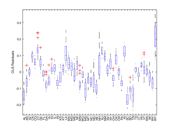
The boxplot of OLS residuals by STATE shows that the within state residuals are either all positive or all negative and are not centred at 0. This violates the fundamental assumption of OLS and the resulting inference may not be valid.
Fixed-Effects Model
Fixed-Effect models treat individual effects as fixed but unknown parameters, so as to allow the unobserved individual effects to be correlated with the included variables. Panel Data Fixed-Effect models also refer to Least Squares with Dummy Variables (LSDV) models. All the state-specific information is incorporated in the dummy variables. fitlm automatically does this under the hood, and it is ideal for fixed-effect models with a moderate number of cross-sectional units.
lm_fe = fitlm(publicdata,...
    'log_GDP ~ 1 + UNEMP + log_PUB_CAP + log_PVT_CAP + log_EMP + STATE')

disp(' '),
disp(['log_PUB_CAP OLS Estimate:  ', num2str(lm_ols.Coefficients{'log_PUB_CAP',1})])
disp(['log_PUB_CAP FE  Estimate: ', num2str(lm_fe.Coefficients{'log_PUB_CAP',1})])
lm_fe =


Linear regression model:
    log_GDP ~ 1 + STATE + UNEMP + log_PUB_CAP + log_PVT_CAP + log_EMP

Estimated Coefficients:
                    Estimate         SE         tStat        pValue
                   __________    __________    ________    ___________

    (Intercept)        2.2016         0.176      12.509     8.5462e-33
    STATE_AR         0.061399       0.01672      3.6722     0.00025726
    STATE_AZ          0.16647      0.013634       12.21     1.8928e-31
    STATE_CA          0.29881      0.036815      8.1164     1.9175e-15
    STATE_CO          0.19429      0.013746      14.135     1.8158e-40
    STATE_CT          0.26959      0.018807      14.334      1.903e-41
    STATE_DE          0.21184      0.022432       9.444     4.2496e-20
    STATE_FL          0.13154      0.020489      6.4198     2.3943e-10
    STATE_GA         0.056591      0.016073       3.521     0.00045546
    STATE_IA          0.12555      0.014002      8.9666     2.3216e-18
    STATE_ID           0.1368      0.025164      5.4363     7.3251e-08
    STATE_IL           0.1857      0.024067      7.7161     3.7521e-14
    STATE_IN         0.057766      0.014086       4.101     4.5557e-05
    STATE_KS           0.1371      0.015636      8.7683     1.1666e-17
    STATE_KY          0.19767         0.014      14.119     2.1724e-40
    STATE_LA          0.31305       0.02213      14.146     1.6006e-40
    STATE_MA           0.1606       0.02308      6.9586     7.3977e-12
    STATE_MD          0.19866      0.020253      9.8092     1.7882e-21
    STATE_ME         0.066799      0.025235       2.647       0.008287
    STATE_MI          0.21538       0.02168      9.9344     5.9093e-22
    STATE_MN          0.11393      0.016549      6.8845     1.2107e-11
    STATE_MO          0.11201      0.015263      7.3384     5.5345e-13
    STATE_MS         0.048408      0.014256      3.3955     0.00072041
    STATE_MT          0.14654      0.026661      5.4962     5.2903e-08
    STATE_NC         0.036009      0.016971      2.1217        0.03418
    STATE_ND          0.14228      0.029669      4.7955     1.9508e-06
    STATE_NE          0.10966      0.016396      6.6883     4.3605e-11
    STATE_NH          0.12253      0.027357       4.479     8.6463e-06
    STATE_NJ          0.24125      0.020144      11.977     2.0566e-30
    STATE_NM          0.25276      0.022268      11.351     1.0563e-27
    STATE_NV          0.14027      0.024615      5.6986     1.7244e-08
    STATE_NY          0.27437      0.038809      7.0699     3.5037e-12
    STATE_OH          0.12103      0.022762      5.3171     1.3856e-07
    STATE_OK          0.21432      0.016437      13.039     3.1226e-35
    STATE_OR          0.14929      0.013996      10.666     7.4331e-25
    STATE_PA         0.087726      0.024799      3.5375     0.00042837
    STATE_RI          0.18673      0.030334      6.1559     1.2049e-09
    STATE_SC        -0.082223      0.016847     -4.8806     1.2881e-06
    STATE_SD         0.088063      0.023997      3.6697     0.00025968
    STATE_TN         0.027481      0.015532      1.7693       0.077245
    STATE_TX          0.19204      0.025172      7.6292     7.0358e-14
    STATE_UT          0.12704      0.017077      7.4394      2.725e-13
    STATE_VA          0.17885      0.018246      9.8022     1.9006e-21
    STATE_VT          0.13458      0.028763       4.679      3.409e-06
    STATE_WA          0.24516      0.020582      11.912     3.9728e-30
    STATE_WI          0.12734      0.017036       7.475     2.1186e-13
    STATE_WV         0.091533      0.018279      5.0077     6.8458e-07
    STATE_WY          0.44694      0.039891      11.204     4.4053e-27
    UNEMP          -0.0052977    0.00098873     -5.3582     1.1139e-07
    log_PUB_CAP      -0.02615      0.029002    -0.90166        0.36752
    log_PVT_CAP       0.29201       0.02512      11.625     7.0751e-29
    log_EMP           0.76816      0.030092      25.527    2.0215e-104


Number of observations: 816, Error degrees of freedom: 764
Root Mean Squared Error: 0.0381
R-squared: 0.999,  Adjusted R-Squared: 0.999
F-statistic vs. constant model: 1.14e+04, p-value = 0

log_PUB_CAP OLS Estimate:  0.15501
log_PUB_CAP FE  Estimate: -0.02615
Notice that the output contains coefficient estimates for each state. In contrast to OLS, the LSDV model reports that public capital is not as economically significant (log_PUB_CAP: -0.02) However, disadvantages to this approach include loss in degrees of freedom when there are a large number of groups and therefore a large number of estimated fixed parameters. The complexity of this model then increases linearly with the number of STATEs. This can be a problem when dealing with a smaller set of observations.
One-Way Random effects Model (Mixed-Effect Model)
Group-specific effects can be modelled using random effects. The state-specific observations in this example are assumed drawn at random from a population. fitlme uses Maximum Likelihood (ML) or Restricted Maximum Likelihood (REML) estimation to compute the coefficients.
lme_oneway = fitlme(publicdata,...
   'log_GDP ~ 1 + log_PUB_CAP + log_PVT_CAP + log_EMP + UNEMP + (1 | STATE)',...
   'FitMethod','REML')

disp(' ')
disp(['log_PUB_CAP OLS Estimate:  ', num2str(lm_ols.Coefficients{'log_PUB_CAP',1})])
disp(['log_PUB_CAP  FE Estimate: ', num2str(lm_fe.Coefficients{'log_PUB_CAP',1})])
disp(['log_PUB_CAP  RE Estimate:  ', num2str(lme_oneway.Coefficients{3,2})])
lme_oneway =


Linear mixed-effects model fit by REML

Model information:
    Number of observations             816
    Fixed effects coefficients           5
    Random effects coefficients         48
    Covariance parameters                2

Formula:
    log_GDP ~ 1 + UNEMP + log_PUB_CAP + log_PVT_CAP + log_EMP + (1 | STATE)

Model fit statistics:
    AIC        BIC        LogLikelihood    Deviance
    -2750.7    -2717.8    1382.4           -2764.7

Fixed effects coefficients (95% CIs):
    Name                   Estimate     SE            tStat       DF
    {'(Intercept)'}           2.1493        0.1357      15.839    811
    {'UNEMP'      }        -0.006116    0.00091025      -6.719    811
    {'log_PUB_CAP'}        0.0023163       0.02365    0.097941    811
    {'log_PVT_CAP'}          0.30933      0.020082      15.404    811
    {'log_EMP'    }          0.73241      0.025211      29.051    811


    pValue         Lower         Upper
     1.9677e-49         1.883        2.4157
     3.4438e-11    -0.0079028    -0.0043293
          0.922     -0.044106      0.048739
     3.7475e-47       0.26991       0.34875
    9.6728e-128       0.68292       0.78189

Random effects covariance parameters (95% CIs):
Group: STATE (48 Levels)
    Name1                  Name2                  Type           Estimate
    {'(Intercept)'}        {'(Intercept)'}        {'std'}        0.087071


    Lower       Upper
    0.070498    0.10754

Group: Error
    Name               Estimate    Lower       Upper
    {'Res Std'}        0.038157    0.036289    0.04012


log_PUB_CAP OLS Estimate:  0.15501
log_PUB_CAP  FE Estimate: -0.02615
log_PUB_CAP  RE Estimate:  0.0023163
In contrast to OLS, a mixed-effect model with STATE specific random effect finds that public capital is economically insignificant in the state's private production (log_PUB_CAP: 0.0023).
Mixed-Effects models such as the one above are also known as error component models, random co-efficient regression models, covariance structure models, or multilevel models. The Statistics Toolbox follows the Mixed-Effects terminology, where the regression model consists of two separate parts, fixed effects and random effects. Fixed-effects terms are the conventional linear regression part, and the random effects are associated with group and are assumed to have a prior distribution.
One-Way Random Effects Model with different predictors
An important aspect of building an accurate predictive model it to choose the right set of predictors. We can attempt to improve the existing random-effects model by including HWY, WATER and UTIL as separate predictors instead of PUB_CAP.
Recall that PUB_CAP = HWY + WATER + UTIL
clc
lme_oneway_new = fitlme(publicdata,...
    ['log_GDP ~ 1 + log_HWY + log_WATER + log_UTIL + log_PVT_CAP +'...
    'log_EMP + UNEMP + (1 | STATE)'],'FitMethod','REML')
lme_oneway_new =


Linear mixed-effects model fit by REML

Model information:
    Number of observations             816
    Fixed effects coefficients           7
    Random effects coefficients         48
    Covariance parameters                2

Formula:
    Linear Mixed Formula with 7 predictors.

Model fit statistics:
    AIC        BIC        LogLikelihood    Deviance
    -2787.7    -2745.5    1402.9           -2805.7

Fixed effects coefficients (95% CIs):
    Name                   Estimate      SE            tStat      DF
    {'(Intercept)'}            2.1782       0.14939     14.581    809
    {'UNEMP'      }        -0.0057842    0.00089788    -6.4421    809
    {'log_HWY'    }          0.062865      0.022921     2.7427    809
    {'log_WATER'  }           0.07543      0.014041     5.3722    809
    {'log_UTIL'   }          -0.10099       0.01716    -5.8853    809
    {'log_PVT_CAP'}            0.2694      0.020855     12.917    809
    {'log_EMP'    }            0.7557      0.025775     29.319    809


    pValue         Lower         Upper
     6.2342e-43         1.885        2.4715
     2.0208e-10    -0.0075466    -0.0040218
      0.0062284      0.017874       0.10786
     1.0178e-07      0.047869       0.10299
     5.8166e-09      -0.13468      -0.06731
     7.7082e-35       0.22846       0.31033
    2.6003e-129       0.70511        0.8063

Random effects covariance parameters (95% CIs):
Group: STATE (48 Levels)
    Name1                  Name2                  Type           Estimate
    {'(Intercept)'}        {'(Intercept)'}        {'std'}        0.089868


    Lower      Upper
    0.07251    0.11138

Group: Error
    Name               Estimate    Lower       Upper
    {'Res Std'}        0.036808    0.035003    0.038706
The log_HWY, log_WATER and log_UTIL estimates are statistically significant. log_UTIL appears to have a negative economic impact on the states private capital.
Compare the two One-Way Random Effects models for improvements
clc
compare(lme_oneway, lme_oneway_new)
ans =


    THEORETICAL LIKELIHOOD RATIO TEST

    Model             DF    AIC        BIC        LogLik    LRStat    deltaDF
    lme_oneway        7     -2750.7    -2717.8    1382.4
    lme_oneway_new    9     -2787.7    -2745.5    1402.9    41.043    2


    pValue

    1.2234e-09
p-Value of the likelihood ratio test is close to zero. This indicates that the random effect model is significantly better than the pure fixed-effect model. Since the p-Value of the log_PUB_CAP estimate in the random-effects model is not significant, we can attempt to improve the model.
Two-Way Random effects Model (Mixed-Effect Model)
The two-way random-effects model takes into account the random effect with time as the grouping variable which is individual-invariant. This accounts for any time-specific effect that is not included in the regression. Economically this could account for events that are specific to a year that affect the state private production.
clc
lme_twoway = fitlme(publicdata,...
    ['log_GDP ~ 1 + log_HWY + log_WATER + log_UTIL + log_PVT_CAP +'...
    'log_EMP + UNEMP + (1 | STATE) + (1|YR)'],'FitMethod','REML')

compare(lme_oneway, lme_twoway)
lme_twoway =


Linear mixed-effects model fit by REML

Model information:
    Number of observations             816
    Fixed effects coefficients           7
    Random effects coefficients         65
    Covariance parameters                3

Formula:
    Linear Mixed Formula with 8 predictors.

Model fit statistics:
    AIC        BIC        LogLikelihood    Deviance
    -2876.3    -2829.3    1448.1           -2896.3

Fixed effects coefficients (95% CIs):
    Name                   Estimate      SE           tStat      DF
    {'(Intercept)'}            2.4129      0.15442     15.626    809
    {'UNEMP'      }        -0.0042953    0.0010625    -4.0428    809
    {'log_HWY'    }           0.08226     0.024747      3.324    809
    {'log_WATER'  }          0.057152     0.013744     4.1583    809
    {'log_UTIL'   }         -0.090081     0.016155    -5.5759    809
    {'log_PVT_CAP'}            0.2212     0.022162      9.981    809
    {'log_EMP'    }            0.7751     0.024684     31.401    809


    pValue         Lower         Upper
     2.6764e-48        2.1098         2.716
     5.7872e-05    -0.0063809    -0.0022098
     0.00092711      0.033684       0.13084
     3.5486e-05      0.030174      0.084131
     3.3564e-08      -0.12179      -0.05837
     3.3338e-22        0.1777        0.2647
    3.7471e-142       0.72664       0.82355

Random effects covariance parameters (95% CIs):
Group: STATE (48 Levels)
    Name1                  Name2                  Type           Estimate
    {'(Intercept)'}        {'(Intercept)'}        {'std'}        0.093399


    Lower       Upper
    0.075159    0.11606

Group: YR (17 Levels)
    Name1                  Name2                  Type           Estimate
    {'(Intercept)'}        {'(Intercept)'}        {'std'}        0.015926


    Lower       Upper
    0.010685    0.023737

Group: Error
    Name               Estimate    Lower       Upper
    {'Res Std'}        0.033774    0.032096    0.035541


ans =


    THEORETICAL LIKELIHOOD RATIO TEST

    Model         DF    AIC        BIC        LogLik    LRStat    deltaDF
    lme_oneway     7    -2750.7    -2717.8    1382.4
    lme_twoway    10    -2876.3    -2829.3    1448.1    131.59    3


    pValue

    0
The likelihood ratio test shows that the two-way random effects model is significantly better than the one-way random-effects model.
Multilevel (Hierarchical) Model: STATE nested in REGION
So far we built models that accounted for state-specific contextual information by introducing random effects for each state. This model can be extended to introduce random effects for STATE and REGION. In this example, STATE is nested within REGION. In other words, groups of states form a region and no state-level observation is part of more than one region. This can be done by including a random effect for REGION (9 levels) and a random effect for the interaction term STATE.*REGION (48 levels).
clc
lme_hierarchical = fitlme(publicdata,...
    ['log_GDP ~ 1 + log_HWY + log_WATER + log_UTIL + log_PVT_CAP +'...
    'log_EMP + UNEMP + (1|REGION) + (1|STATE:REGION) + (1|YR)'],'FitMethod','REML')
lme_hierarchical =


Linear mixed-effects model fit by REML

Model information:
    Number of observations             816
    Fixed effects coefficients           7
    Random effects coefficients         74
    Covariance parameters                4

Formula:
    Linear Mixed Formula with 9 predictors.

Model fit statistics:
    AIC        BIC        LogLikelihood    Deviance
    -2878.2    -2826.5    1450.1           -2900.2

Fixed effects coefficients (95% CIs):
    Name                   Estimate      SE           tStat      DF
    {'(Intercept)'}            2.3928      0.16409     14.582    809
    {'UNEMP'      }        -0.0043974    0.0010682    -4.1168    809
    {'log_HWY'    }          0.089372     0.024872     3.5933    809
    {'log_WATER'  }          0.058102     0.013688     4.2446    809
    {'log_UTIL'   }         -0.089943     0.016032    -5.6101    809
    {'log_PVT_CAP'}           0.21538     0.022801     9.4461    809
    {'log_EMP'    }           0.77702     0.025223     30.806    809


    pValue         Lower         Upper
     6.2072e-43        2.0707        2.7149
     4.2365e-05    -0.0064941    -0.0023007
     0.00034626      0.040551       0.13819
     2.4433e-05      0.031233      0.084971
     2.7777e-08      -0.12141     -0.058473
     3.6701e-20       0.17062       0.26013
    1.7222e-138       0.72751       0.82653

Random effects covariance parameters (95% CIs):
Group: REGION (9 Levels)
    Name1                  Name2                  Type           Estimate
    {'(Intercept)'}        {'(Intercept)'}        {'std'}        0.047011


    Lower       Upper
    0.020556    0.10751

Group: STATE:REGION (48 Levels)
    Name1                  Name2                  Type           Estimate
    {'(Intercept)'}        {'(Intercept)'}        {'std'}        0.082574


    Lower       Upper
    0.065183    0.10461

Group: YR (17 Levels)
    Name1                  Name2                  Type           Estimate
    {'(Intercept)'}        {'(Intercept)'}        {'std'}        0.016016


    Lower       Upper
    0.010731    0.023903

Group: Error
    Name               Estimate    Lower       Upper
    {'Res Std'}        0.033772    0.032093    0.035537
Regional random effects for UNEMP and HWY with possible correlation
lme_advanced = fitlme(publicdata,...
    ['log_GDP ~ 1 + log_HWY + log_WATER + log_UTIL + log_PVT_CAP + log_EMP + UNEMP +'...
    '(1 + log_HWY + UNEMP|REGION) + (1 + log_HWY + UNEMP|STATE:REGION) + (1|YR)'],...
    'FitMethod','REML','CovariancePattern',{'Full','Diagonal','Diagonal'})
compare(lme_hierarchical, lme_advanced,'CheckNesting',true)
lme_advanced =


Linear mixed-effects model fit by REML

Model information:
    Number of observations             816
    Fixed effects coefficients           7
    Random effects coefficients        188
    Covariance parameters               11

Formula:
    Linear Mixed Formula with 9 predictors.

Model fit statistics:
    AIC        BIC        LogLikelihood    Deviance
    -2999.8    -2915.3    1517.9           -3035.8

Fixed effects coefficients (95% CIs):
    Name                   Estimate      SE           tStat      DF
    {'(Intercept)'}            2.5426      0.42123     6.0362    809
    {'UNEMP'      }        -0.0042169    0.0020824     -2.025    809
    {'log_HWY'    }          0.079243     0.048999     1.6172    809
    {'log_WATER'  }          0.035572     0.013372     2.6603    809
    {'log_UTIL'   }          -0.05954        0.017    -3.5024    809
    {'log_PVT_CAP'}           0.16467     0.022807       7.22    809
    {'log_EMP'    }           0.83055     0.026705     31.101    809


    pValue         Lower         Upper
     2.4023e-09        1.7158         3.3695
       0.043197    -0.0083044    -0.00012929
        0.10622     -0.016937        0.17542
      0.0079629     0.0093247       0.061819
     0.00048641     -0.092909      -0.026171
        1.2e-12        0.1199        0.20944
    2.6314e-140       0.77813        0.88297

Random effects covariance parameters (95% CIs):
Group: REGION (9 Levels)
    Name1                  Name2                  Type            Estimate
    {'(Intercept)'}        {'(Intercept)'}        {'std' }           1.0807
    {'UNEMP'      }        {'(Intercept)'}        {'corr'}         -0.07628
    {'log_HWY'    }        {'(Intercept)'}        {'corr'}         -0.99583
    {'UNEMP'      }        {'UNEMP'      }        {'std' }        0.0042097
    {'log_HWY'    }        {'UNEMP'      }        {'corr'}         -0.01499
    {'log_HWY'    }        {'log_HWY'    }        {'std' }           0.1175


    Lower        Upper
       0.6534       1.7874
     -0.11649    -0.035823
     -0.99589     -0.99577
    0.0020541    0.0086273
    -0.055524     0.025593
     0.070978       0.1945

Group: STATE:REGION (48 Levels)
    Name1                  Name2                  Type           Estimate
    {'(Intercept)'}        {'(Intercept)'}        {'std'}           0.13535
    {'UNEMP'      }        {'UNEMP'      }        {'std'}         0.0069407
    {'log_HWY'    }        {'log_HWY'    }        {'std'}        9.4345e-06


    Lower        Upper
       0.1034      0.17718
    0.0051992    0.0092654
          NaN          NaN

Group: YR (17 Levels)
    Name1                  Name2                  Type           Estimate
    {'(Intercept)'}        {'(Intercept)'}        {'std'}        0.01954


    Lower       Upper
    0.013218    0.028887

Group: Error
    Name               Estimate    Lower       Upper
    {'Res Std'}        0.028184    0.026673    0.029781


ans =


    THEORETICAL LIKELIHOOD RATIO TEST

    Model               DF    AIC        BIC        LogLik    LRStat    deltaDF
    lme_hierarchical    11    -2878.2    -2826.5    1450.1
    lme_advanced        18    -2999.8    -2915.3    1517.9    135.62    7


    pValue

    0
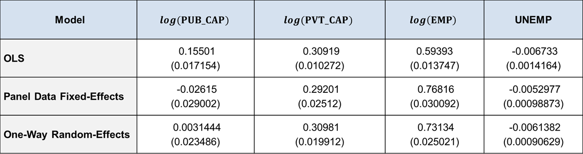
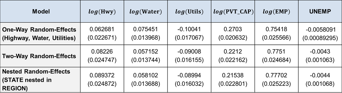
Table showing Cobb–Douglas Production Function Estimates for different models


Bibliography
This example is based on the following literature:
[1] Alicia H. Munnell & Leah M. Cook, 1990. "How does public infrastructure affect regional economic performance?," New England Economic Review, Federal Reserve Bank of Boston, issue Sep, pages 11-33.
[2] Econometric Analysis of Panel Data, 5th Edition, Badi H. Baltagi


Comments