Checking the outlier of the data
Posted by: admin 1 year, 3 months ago
(Comments)

We know there is always no average data in data; it can be from the wrong input data.
A single observation that is substantially different from all other observations can make a significant difference in the results of your regression analysis. If a single observation (or small group of observations) substantially changes your results, you would want to know about this and investigate further. There are three ways that an observation can be unusual.
Outliers: In linear regression, an outlier is an observation with a large residual. In other words, it is an observation whose dependent-variable value is unusual given its values on the predictor variables. An outlier may indicate a sample peculiarity or a data entry error or another problem.
Leverage: An observation with an extreme value on a predictor variable is a point with high leverage. Leverage is a measure of how far an observation deviates from the mean
of that variable. These leverage points can affect the estimate of regression coefficients.
Influence: An observation is said to be influential if removing the observation substantially changes the estimate of coefficients. Influence can be thought of as the product of leverage and outliers.
How can we identify these three types of observations? Let’s look at an example dataset called crime. This dataset appears in Statistical Methods for Social Sciences, Third Edition by Alan Agresti and Barbara Finlay (Prentice Hall, 1997). The variables are state id (sid), state name (state), violent crimes per 100,000 people (crime), murders per 1,000,000 (murder), the percent of the population living in metropolitan areas (pctmetro), the percent of the population that is white (pctwhite), percent of the population with a high school education or above (pcths), percent of the population living under the poverty line (poverty), and percent of the population that is single parents (single).
use https://stats.idre.ucla.edu/stat/stata/webbooks/reg/crime
	(crime data from agresti & finlay - 1997)

describe

Contains data from crime.dta
  obs:            51                          crime data from agresti &
                                                finlay - 1997
 vars:            11                          6 Feb 2001 13:52
 size:         2,295 (98.9% of memory free)
-------------------------------------------------------------------------------
   1. sid       float  %9.0g
   2. state     str3   %9s
   3. crime     int    %8.0g                  violent crime rate
   4. murder    float  %9.0g                  murder rate
   5. pctmetro  float  %9.0g                  pct metropolitan
   6. pctwhite  float  %9.0g                  pct white
   7. pcths     float  %9.0g                  pct hs graduates
   8. poverty   float  %9.0g                  pct poverty
   9. single    float  %9.0g                  pct single parent
-------------------------------------------------------------------------------
Sorted by:

summarize crime murder pctmetro pctwhite pcths poverty single

Variable |     Obs        Mean   Std. Dev.       Min        Max
---------+-----------------------------------------------------
   crime |      51    612.8431   441.1003         82       2922
  murder |      51    8.727451   10.71758        1.6       78.5
pctmetro |      51     67.3902   21.95713         24        100
pctwhite |      51    84.11569   13.25839       31.8       98.5
   pcths |      51    76.22353   5.592087       64.3       86.6
 poverty |      51    14.25882   4.584242          8       26.4
  single |      51    11.32549   2.121494        8.4       22.1
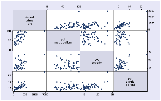
Let’s say we want to predict crime by pctmetro, poverty, and single. That is to say, we want to build a linear regression model between the response variable crime and the independent variables pctmetro, poverty and single. We will first look at the scatter plots of crime against each of the predictor variables before the regression analysis so we will have some ideas about potential problems. We can create a scatterplot matrix of these variables as shown below.
graph matrix crime pctmetro poverty single
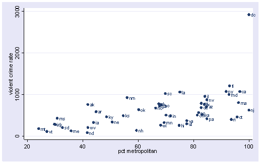
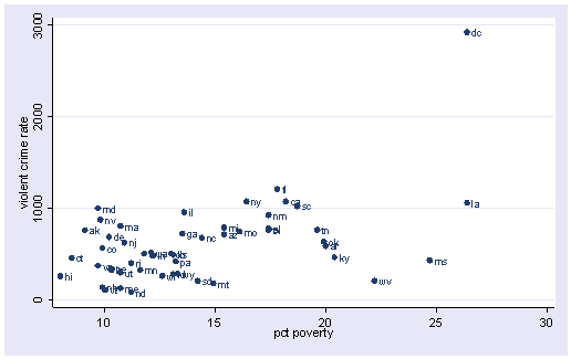
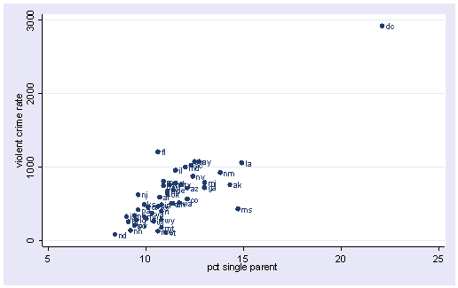
The graphs of crime with other variables show some potential problems. In every plot, we see a data point that is far away from the rest of the data points. Let’s make individual graphs of crime with pctmetro and poverty and single so we can better view these scatterplots. We will add the mlabel(state) option to label each marker with the state name to identify outlying states.
scatter crime pctmetro, mlabel(state)
scatter crime poverty, mlabel(state)
scatter crime single, mlabel(state)
All the scatter plots suggest that the observation for state = dc is a point that requires extra attention since it stands out away from all of the other points. We will keep it in mind when we do our regression analysis.
Now let’s try the regression command predicting crime from pctmetro poverty and single. We will go step-by-step to identify all the potentially unusual or influential points afterwards.
regress crime pctmetro poverty single

  Source |       SS       df       MS                  Number of obs =      51
---------+------------------------------               F(  3,    47) =   82.16
   Model |  8170480.21     3  2723493.40               Prob > F      =  0.0000
Residual |  1557994.53    47  33148.8199               R-squared     =  0.8399
---------+------------------------------               Adj R-squared =  0.8296
   Total |  9728474.75    50  194569.495               Root MSE      =  182.07

------------------------------------------------------------------------------
   crime |      Coef.   Std. Err.       t     P>|t|       [95% Conf. Interval]
---------+--------------------------------------------------------------------
pctmetro |   7.828935   1.254699      6.240   0.000       5.304806    10.35306
 poverty |   17.68024    6.94093      2.547   0.014       3.716893    31.64359
  single |   132.4081   15.50322      8.541   0.000       101.2196    163.5965
   _cons |  -1666.436    147.852    -11.271   0.000      -1963.876   -1368.996
------------------------------------------------------------------------------
Let’s examine the studentized residuals as the first means for identifying outliers. Below we use the predict command with the rstudent option to generate studentized residuals, and we name the residuals r. We can choose any name we like as long as it is a legal Stata variable. Studentized residuals are a type of standardized residual that can be used to identify outliers.
predict r, rstudent
Let’s examine the residuals with a stem and leaf plot. We see three residuals that stick out, -3.57, 2.62 and 3.77.
stem r

Stem-and-leaf plot for r (Studentized residuals)

r rounded to nearest multiple of .01
plot in units of .01

-3** | 57
-3** |
-2** |
-2** |
-1** | 84,69
-1** | 30,15,13,04,02
-0** | 87,85,65,58,56,55,54
-0** | 47,46,45,38,36,30,28,21,08,02
 0** | 05,06,08,13,27,28,29,31,35,41,48,49
 0** | 56,64,70,80,82
 1** | 01,03,03,08,15,29
 1** | 59
 2** |
 2** | 62
 3** |
 3** | 77
The stem and leaf display helps us see potential outliers, but we cannot see which state (which observations) are potential outliers. Let’s sort the data on the residuals and show the 10 most significant and 10 smallest residuals along with the state id and name. Note that in the second list command, the -10/l the last value is the letter “l”, NOT the number one.
sort r
list sid state r in 1/10

           sid      state          r
  1.        25         ms  -3.570789
  2.        18         la  -1.838577
  3.        39         ri  -1.685598
  4.        47         wa  -1.303919
  5.        35         oh   -1.14833
  6.        48         wi   -1.12934
  7.         6         co  -1.044952
  8.        22         mi  -1.022727
  9.         4         az  -.8699151
 10.        44         ut  -.8520518

list sid state r in -10/l

           sid      state          r
 42.        24         mo   .8211724
 43.        20         md    1.01299
 44.        29         ne   1.028869
 45.        40         sc   1.030343
 46.        16         ks   1.076718
 47.        14         il   1.151702
 48.        13         id   1.293477
 49.        12         ia   1.589644
 50.         9         fl   2.619523
 51.        51         dc   3.765847
We should pay attention to studentized residuals that exceed +2 or -2, and get even more concerned about residuals that exceed +2.5 or -2.5 and even yet more concerned about residuals that exceed +3 or -3. These results show that DC and MS are the most worrisome observations followed by FL.
Another way to get this kind of output is with a command called hilo. You can download hilo from within Stata by typing search hilo (see How can I used the search command to search for programs and get additional help? for more information about using search).
Once installed, you can type the following and get output similar to that above by typing just one command.
hilo r state10 smallest and largest observations on r r state -3.570789 ms -1.838577 la -1.685598 ri -1.303919 wa -1.14833 oh -1.12934 wi -1.044952 co -1.022727 mi -.8699151 az -.8520518 ut r state 8211724 mo 1.01299 md 1.028869 ne 1.030343 sc 1.076718 ks 1.151702 il 1.293477 id 1.589644 ia 2.619523 fl 3.765847 dc
Let’s show all of the variables in our regression where the studentized residual exceeds +2 or -2, i.e., where the absolute value of the residual exceeds 2. We see the data for the three potential outliers we identified, namely Florida, Mississippi, and Washington D.C. Looking carefully at these three observations, we couldn’t find any data entry error, though we may want to do another regression analysis with the extreme point such as DC deleted. We will return to this issue later.
list r crime pctmetro poverty single if abs(r) > 2

             r     crime   pctmetro    poverty     single
  1. -3.570789       434       30.7       24.7       14.7
 50.  2.619523      1206         93       17.8       10.6
 51.  3.765847      2922        100       26.4       22.1
Now let’s look at the leverage to identify observations that will have a potential significant influence on regression coefficient estimates.
predict lev, leverage
stem lev

Stem-and-leaf plot for l (Leverage)

l rounded to nearest multiple of .001
plot in units of .001

  0** | 20,24,24,28,29,29,31,31,32,32,34,35,37,38,39,43,45,45,46,47,49
  0** | 50,57,60,61,62,63,63,64,64,67,72,72,73,76,76,82,83,85,85,85,91,95
  1** | 00,02,36
  1** | 65,80,91
  2** |
  2** | 61
  3** |
  3** |
  4** |
  4** |
  5** | 36
We use the show(5) high options on the hilo command to show just the 5 largest observations (the high option can be abbreviated as h). We see that DC has the largest leverage.
hilo lev state, show(5) high

5 largest observations on lev

      lev      state
.1652769         la
.1802005         wv
 .191012         ms
.2606759         ak
 .536383         dc
Generally, a point with leverage greater than (2k+2)/n should be carefully examined. Here k is the number of predictors and n is the number of observations. In our example, we can do the following.
display (2*3+2)/51
.15686275

list crime pctmetro poverty single state lev if lev >.156

        crime   pctmetro    poverty     single      state   lev
  5.      208       41.8       22.2        9.4         wv   .1802005
 48.      761       41.8        9.1       14.3         ak   .2606759
 49.      434       30.7       24.7       14.7         ms    .191012
 50.     1062         75       26.4       14.9         la   .1652769
 51.     2922        100       26.4       22.1         dc    .536383
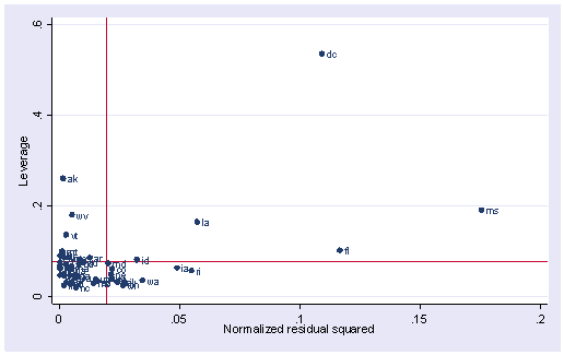
As we have seen, DC is an observation that both have a significant residual and large leverage. Such points are potentially the most influential. We can make a plot showing the leverage by the residual squared and look for jointly high observations on both of these measures. We can do this using the lvr2plot command. lvr2plot stands for leverage versus residual squared plot. Using residually squared instead of residual itself, the graph is restricted to the first quadrant, and the relative positions of data points are preserved. This is a quick way of simultaneously checking potential, influential observations, and outliers. Both types of points are of great concern to us.
lvr2plot, mlabel(state)
The two reference lines are the means for leverage, horizontal, and for the normalized residual squared, vertical. The points that immediately catch our attention is DC (with the largest leverage) and MS (with the largest residual squared). We’ll look at those observations more carefully by listing them.
list state crime pctmetro poverty single if state=="dc" | state=="ms"

         state     crime   pctmetro    poverty     single
 49.        ms       434       30.7       24.7       14.7
 51.        dc      2922        100       26.4       22.1
Now let’s move on to overall influence measures, specifically at Cook’s D and DFITS. These measures both combine information on the residual and leverage. Cook’s D and DFITS are very similar, except that they scale differently but give us similar answers.
The lowest value that Cook’s D can assume is zero, and the higher the Cook’s D is, the more influential the point. The convention cut-off point is 4/n. We can list any observation above the cut-off point by doing the following. We see that Cook’s D for DC is by far the largest.
predict d, cooksd
list crime pctmetro poverty single state d if d>4/51

        crime   pctmetro    poverty     single      state          d
  1.      434       30.7       24.7       14.7         ms    .602106
  2.     1062         75       26.4       14.9         la   .1592638
 50.     1206         93       17.8       10.6         fl    .173629
 51.     2922        100       26.4       22.1         dc   3.203429
Now let’s take a look at DFITS. The cut-off point for DFITS is 2*sqrt(k/n). DFITS can be either positive or negative, with numbers close to zero corresponding to the points with small or zero influence. As we see, dfit also indicates that DC is, by far, the most influential observation.
predict dfit, dfits
list crime pctmetro poverty single state dfit if abs(dfit)>2*sqrt(3/51)

        crime   pctmetro    poverty     single      state       dfit
 18.     1206         93       17.8       10.6         fl   .8838196
 49.      434       30.7       24.7       14.7         ms  -1.735096
 50.     1062         75       26.4       14.9         la  -.8181195
 51.     2922        100       26.4       22.1         dc   4.050611
The above measures are general measures of influence. You can also consider more specific measures of influence that assess how each coefficient is changed by deleting the observation. This measure is called DFBETA and is created for each of the predictors. Apparently this is more computational intensive than summary statistics such as Cook’s D since the more predictors a model has, the more computation it may involve. We can restrict our attention to only those predictors that we are most concerned with to see how well behaved those predictors are. In Stata, the dfbeta command will produce the DFBETAs for each of the predictors. The names for the new variables created are chosen by Stata automatically and begin with the letters DF.
dfbeta
                      DFpctmetro:  DFbeta(pctmetro)
                       DFpoverty:  DFbeta(poverty)
                        DFsingle:  DFbeta(single)
This created three variables, DFpctmetro, DFpoverty and DFsingle. Let’s look at the first 5 values.
list state DFpctmetro DFpoverty DFsingle in 1/5

         state  DFpctme~o  DFpoverty   DFsingle
  1.        ak  -.1061846  -.1313398   .1451826
  2.        al   .0124287   .0552852  -.0275128
  3.        ar  -.0687483   .1753482  -.1052626
  4.        az  -.0947614  -.0308833    .001242
  5.        ca   .0126401   .0088009  -.0036361
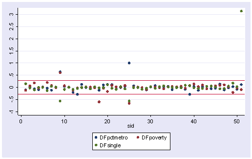
The value for DFsingle for Alaska is .14, which means that by being included in the analysis (as compared to being excluded), Alaska increases the coefficient for single by 0.14 standard errors, i.e., .14 times the standard error for BSingle or by (0.14 * 15.5). Since the inclusion of an observation could either contribute to an increase or decrease in a regression coefficient, DFBETAs can be either positive or negative. A DFBETA value in excess of 2/sqrt(n) merits further investigation. In this example, we would be concerned about absolute values in excess of 2/sqrt(51) or .28.
We can plot all three DFBETA values against the state id in one graph shown below. We add a line at .28 and -.28 to help us see potentially troublesome observations. We see the largest value is about 3.0 for DFsingle.
scatter DFpctmetro DFpoverty DFsingle sid, ylabel(-1(.5)3) yline(.28 -.28)
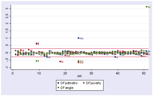
We can repeat this graph with the mlabel() option in the graph command to label the points. With the graph above we can identify which DFBeta is a problem, and with the graph below we can associate that observation with the state that it originates from.
scatter DFpctmetro DFpoverty DFsingle sid, ylabel(-1(.5)3) yline(.28 -.28) ///
  mlabel(state state state)
Now let’s list those observations with DFsingle larger than the cut-off value.
list DFsingle state crime pctmetro poverty single if abs(DFsingle) > 2/sqrt(51)

      DFsingle      state     crime   pctmetro    poverty     single
  9. -.5606022         fl      1206         93       17.8       10.6
 25. -.5680245         ms       434       30.7       24.7       14.7
 51.  3.139084         dc      2922        100       26.4       22.1
The following table summarizes the general rules of thumb we use for these measures to identify observations worthy of further investigation (where k is the number of predictors and n is the number of observations).
| Measure | Value |
| leverage | >(2k+2)/n |
| abs(rstu) | > 2 |
| Cook’s D | > 4/n |
| abs(DFITS) | > 2*sqrt(k/n) |
| abs(DFBETA) | > 2/sqrt(n) |
We have used the predict command to create a number of variables associated with regression analysis and regression diagnostics. The help regress command not only gives help on the regress command, but also lists all of the statistics that can be generated via the predict command. Below we show a snippet of the Stata help file illustrating the various statistics that can be computed via the predict command.
help regress

-------------------------------------------------------------------------------
help for regress                                         (manual:  [R] regress)
-------------------------------------------------------------------------------

<--output omitted-->

The syntax of predict following regress is

        predict [type] newvarname [if exp] [in range] [, statistic]

where statistic is

        xb                           fitted values; the default
        pr(a,b)                      Pr(y |a>y>b)  (a and b may be numbers
        e(a,b)                       E(y |a>y>b)    or variables; a==. means
        ystar(a,b)                   E(y*)          -inf; b==. means inf)
        cooksd                       Cook's distance
        leverage | hat               leverage (diagonal elements of hat matrix)
        residuals                    residuals
        rstandard                    standardized residuals
        rstudent                     Studentized (jackknifed) residuals
        stdp                         standard error of the prediction
        stdf                         standard error of the forecast
        stdr                         standard error of the residual
    (*) covratio                     COVRATIO
    (*) dfbeta(varname)              DFBETA for varname
    (*) dfits                        DFITS
    (*) welsch                       Welsch distance

Unstarred statistics are available both in and out of sample; type "predict ...
if e(sample) ..." if wanted only for the estimation sample.  Starred statistics
are calculated for the estimation sample even when "if e(sample)" is not speci-
fied.

<--more output omitted here.-->
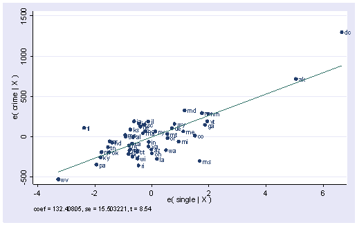
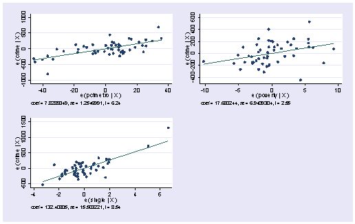
We have explored a number of the statistics that we can get after the regress command. There are also several graphs that can be used to search for unusual and influential observations. The avplot command graphs an added-variable plot. It is also called a partial-regression plot and is very useful in identifying influential points. For example, in the avplot for single shown below, the graph shows crime by single after both crime and single have been adjusted for all other predictors in the model. The line plotted has the same slope as the coefficient for single. This plot shows how the observation for DC influences the coefficient. You can see how the regression line is tugged upwards trying to fit through the extreme value of DC. Alaska and West Virginia may also exert substantial leverage on the coefficient of single.
avplot single, mlabel(state)
Stata also has the avplots command that creates an added variable plot for all of the variables, which can be very useful when you have many variables. It does produce small graphs, but these graphs can quickly reveal whether you have problematic observations based on the added variable plots.
avplots
DC has appeared as an outlier and influential point in every analysis. Since DC is really not a state, we can use this to justify omitting it from the analysis saying that we really wish to just analyze states. First, let’s repeat our analysis including DC by just typing regress.
regress

  Source |       SS       df       MS                  Number of obs =      51
---------+------------------------------               F(  3,    47) =   82.16
   Model |  8170480.21     3  2723493.40               Prob > F      =  0.0000
Residual |  1557994.53    47  33148.8199               R-squared     =  0.8399
---------+------------------------------               Adj R-squared =  0.8296
   Total |  9728474.75    50  194569.495               Root MSE      =  182.07

------------------------------------------------------------------------------
   crime |      Coef.   Std. Err.       t     P>|t|       [95% Conf. Interval]
---------+--------------------------------------------------------------------
pctmetro |   7.828935   1.254699      6.240   0.000       5.304806    10.35306
 poverty |   17.68024    6.94093      2.547   0.014       3.716893    31.64359
  single |   132.4081   15.50322      8.541   0.000       101.2196    163.5965
   _cons |  -1666.436    147.852    -11.271   0.000      -1963.876   -1368.996
------------------------------------------------------------------------------
Now, let’s run the analysis omitting DC by including if state != “dc” on the regress command (here != stands for “not equal to” but you could also use ~= to mean the same thing). As we expect, deleting DC made a large change in the coefficient for single. The coefficient for single dropped from 132.4 to 89.4. After having deleted DC, we would repeat the process we have illustrated in this section to search for any other outlying and influential observations.
regress crime pctmetro poverty single if state!="dc"

  Source |       SS       df       MS                  Number of obs =      50
---------+------------------------------               F(  3,    46) =   39.90
   Model |  3098767.11     3  1032922.37               Prob > F      =  0.0000
Residual |  1190858.11    46  25888.2199               R-squared     =  0.7224
---------+------------------------------               Adj R-squared =  0.7043
   Total |  4289625.22    49  87543.3718               Root MSE      =  160.90

------------------------------------------------------------------------------
   crime |      Coef.   Std. Err.       t     P>|t|       [95% Conf. Interval]
---------+--------------------------------------------------------------------
pctmetro |   7.712334   1.109241      6.953   0.000       5.479547     9.94512
 poverty |   18.28265   6.135958      2.980   0.005       5.931611     30.6337
  single |   89.40078   17.83621      5.012   0.000       53.49836    125.3032
   _cons |  -1197.538   180.4874     -6.635   0.000       -1560.84   -834.2358
------------------------------------------------------------------------------
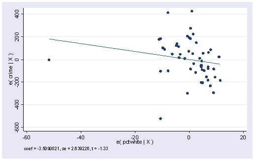
Finally, we showed that the avplot command can be used to searching for outliers among existing variables in your model, but we should note that the avplot command not only works for the variables in the model, it also works for variables that are not in the model, which is why it is called added-variable plot. Let’s use the regression that includes DC as we want to continue to see ill-behavior caused by DC as a demonstration for doing regression diagnostics. We can do an avplot on variable pctwhite.
regress crime pctmetro poverty single
avplot pctwhite
At the top of the plot, we have “coef=-3.509”. It is the coefficient for pctwhite if it were put in the model. We can check that by doing a regression as below.
regress crime pctmetro pctwhite poverty single

  Source |       SS       df       MS                  Number of obs =      51
---------+------------------------------               F(  4,    46) =   63.07
   Model |  8228138.87     4  2057034.72               Prob > F      =  0.0000
Residual |  1500335.87    46  32615.9972               R-squared     =  0.8458
---------+------------------------------               Adj R-squared =  0.8324
   Total |  9728474.75    50  194569.495               Root MSE      =  180.60

------------------------------------------------------------------------------
   crime |      Coef.   Std. Err.       t     P>|t|       [95% Conf. Interval]
---------+--------------------------------------------------------------------
pctmetro |   7.404075   1.284941      5.762   0.000       4.817623    9.990526
pctwhite |  -3.509082   2.639226     -1.330   0.190      -8.821568    1.803404
 poverty |   16.66548   6.927095      2.406   0.020       2.721964      30.609
  single |   120.3576    17.8502      6.743   0.000       84.42702    156.2882
   _cons |  -1191.689   386.0089     -3.087   0.003      -1968.685   -414.6936
------------------------------------------------------------------------------
Summary
In this section, we explored several methods of identifying outliers and influential points. In a typical analysis, you would probably use only some of these methods. Generally speaking, there are two types of methods for assessing outliers: statistics such as residuals, leverage, Cook’s D and DFITS, that assess the overall impact of an observation on the regression results, and statistics such as DFBETA that assess the specific impact of an observation on the regression coefficients.
In our example, we found that DC was a point of major concern. We performed a regression with it and without it and the regression equations were very different. We can justify removing it from our analysis by reasoning that our model is to predict crime rate for states, not for metropolitan areas.
Link

Ready or not, we can not ignore not using regression in our daily activity. Regression also in history already reach 100 years! Lets dig into the requirement to make a regression acceptable. The source is coming from many other sources!
Regression diagnostic consists of a couple of methods
- 2.1 Unusual and Influential data
- 2.2 Checking Normality of Residuals
- 2.3 Checking Homoscedasticity
- 2.4 Checking for Multicollinearity
- 2.5 Checking Linearity
- 2.6 Model Specification
- 2.7 Issues of Independence
- 2.8 Summary
- 2.9 Self-assessment
- 2.10 For more information
Let's see them one by one.
Reference
Regression page
3 months, 3 weeks ago
A reflection of using kanban flow and being minimalist
Recent newsToday is the consecutive day I want to use and be consistent with the Kanban flow! It seems it's perfect to limit my parallel and easily distractedness.
read more4 months ago
4 months ago
Podcast Bapak Dimas 2 - pindahan rumah
Recent newsVlog kali ini adalah terkait pindahan rumah!
read more4 months, 1 week ago
Podcast Bapak Dimas - Bapaknya Jozio dan Kaziu - ep 1
Recent newsSeperti yang saya cerita kan sebelumnya, berikut adalah catatan pribadi VLOG kita! Bapak Dimas
read more4 months, 1 week ago
Happy new year 2024 and thank you 2023!
Recent newsAs the new year starts, I want to revisit what has happened in 2023.
read more4 months, 1 week ago
Some notes about python and Zen of Python
Recent newsExplore Python syntax
Python is a flexible programming language used in a wide range of fields, including software development, machine learning, and data analysis. Python is one of the most popular programming languages for data professionals, so getting familiar with its fundamental syntax and semantics will be useful for your future career. In this reading, you will learn about Python’s syntax and semantics, as well as where to find resources to further your learning.
5 months, 2 weeks ago

Collaboratively administrate empowered markets via plug-and-play networks. Dynamically procrastinate B2C users after installed base benefits. Dramatically visualize customer directed convergence without



Comments