
PhD Chapter - Hodrick Prescott Filter
Posted by: admin 2 years, 4 months ago
(Comments)

This example shows how to use the Hodrick-Prescott filter to decompose a time series.

Hi, my name is Dimas, I am a data enthusiast. At this moment I am writing several chapters related to Big Data, Macroprudential effect on the economy, and a couple of economic and IT research. If you are interested in collaborating, please write your mail to [email protected]
Thanks for stopping by. All the information here is curated from the most inspirational article on the site.
The formula
The Hodrick-Prescott filter separates a time series into growth and cyclical components with
\( y_t = g_t + c_t \)
yt=gt+ct
where yt is a time series, gt is the growth component of yt, and ct is the cyclical component of yt for t=1,...,T.
The objective function for the Hodrick-Prescott filter has the form
Tt=1c2t+λT−1t=2((gt+1−gt)−(gt−gt−1))2
with a smoothing parameter λ. The programming problem is to minimize the objective over all g1,...,gT.
The conceptual basis for this programming problem is that the first sum minimizes the difference between the data and its growth component (which is the cyclical component) and the second sum minimizes the second-order difference of the growth component, which is analogous to minimization of the second derivative of the growth component.
Note that this filter is equivalent to a cubic spline smoother.
Use of the Hodrick-Prescott Filter to Analyze GNP Cyclicality
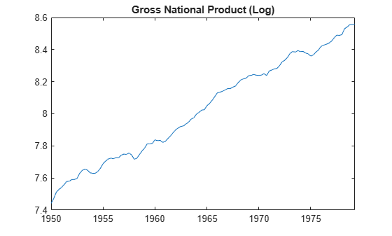
Using data similar to the data found in Hodrick and Prescott [1], plot the cyclical component of GNP. This result should coincide with the results in the paper. However, since the GNP data here and in the paper are both adjusted for seasonal variations with conversion from nominal to real values, differences can be expected due to differences in the sources for the pair of adjustments. Note that our data comes from the St. Louis Federal Reserve FRED database [2], which was downloaded with the Datafeed Toolbox™.
load Data_GNP

startdate = 1950;	% Date range is from 1947.0 to 2005.5 (quarterly)
enddate = 1979.25;	% Change these two lines to try alternative periods

startindex = find(dates == startdate);
endindex = find(dates == enddate);

gnpdates = dates(startindex:endindex);
gnpraw = log(DataTable.GNPR(startindex:endindex));
We run the filter for different smoothing parameters λ = 400, 1600, 6400, and ∞. The infinite smoothing parameter just detrends the data.
[gnptrend4, gnpcycle4] = hpfilter(gnpraw,400);
[gnptrend16, gnpcycle16] = hpfilter(gnpraw,1600);
[gnptrend64, gnpcycle64] = hpfilter(gnpraw,6400);
[gnptrendinf, gnpcycleinf] = hpfilter(gnpraw,Inf);
Plot Cyclical GNP and Its Relationship with Long-Term Trend
The following code generates Figure 1 from Hodrick and Prescott [1].
plot(gnpdates,gnpcycle16,'b');
hold all
plot(gnpdates,gnpcycleinf - gnpcycle16,'r');
title('\bfFigure 1 from Hodrick and Prescott');
ylabel('\bfGNP Growth');
legend('Cyclical GNP','Difference');
hold off
The blue line is the cyclical component with smoothing parameter 1600 and the red line is the difference with respect to the detrended cyclical component. The difference is smooth enough to suggest that the choice of smoothing parameter is appropriate.
Statistical Tests on Cyclical GNP
We will now reconstruct Table 1 from Hodrick and Prescott [1]. With the cyclical components, we compute standard deviations, autocorrelations for lags 1 to 10, and perform a Dickey-Fuller unit root test to assess non-stationarity. As in the article, we see that as lambda increases, standard deviations increase, autocorrelations increase over longer lags, and the unit root hypothesis is rejected for all but the detrended case. Together, these results imply that any of the cyclical series with finite smoothing is effectively stationary.
gnpacf4 = autocorr(gnpcycle4,'NumLags',10);
gnpacf16 = autocorr(gnpcycle16,'NumLags',10);
gnpacf64 = autocorr(gnpcycle64,'NumLags',10);
gnpacfinf = autocorr(gnpcycleinf,'NumLags',10);

[H4, ~, gnptest4] = adftest(gnpcycle4,'Model','ard');
[H16, ~, gnptest16] = adftest(gnpcycle16,'Model','ard');
[H64, ~, gnptest64] = adftest(gnpcycle64,'Model','ard');
[Hinf, ~, gnptestinf] = adftest(gnpcycleinf,'Model','ard');

displayResults(gnpcycle4,gnpcycle16,gnpcycle64,gnpcycleinf,...
    gnpacf4,gnpacf16,gnpacf64,gnpacfinf,...
    gnptest4,gnptest16,gnptest64,gnptestinf,...
    H4,H16,H64,Hinf);
Table 1 from Hodrick and Prescott Reference
              Smoothing Parameter
                     400        1600        6400    Infinity
  Std. Dev.         1.52        1.75        2.06        3.11
  Autocorrelations
           1        0.74        0.78        0.82        0.92
           2        0.38        0.47        0.57        0.81
           3        0.05        0.17        0.33        0.70
           4       -0.21       -0.07        0.12        0.59
           5       -0.36       -0.24       -0.03        0.50
           6       -0.39       -0.30       -0.10        0.44
           7       -0.35       -0.31       -0.13        0.39
           8       -0.28       -0.29       -0.15        0.35
           9       -0.22       -0.26       -0.15        0.31
          10       -0.19       -0.25       -0.17        0.26
  Unit Root        -4.35       -4.13       -3.79       -2.28
  Reject H0            1           1           1           0
Local Function
function displayResults(gnpcycle4,gnpcycle16,gnpcycle64,gnpcycleinf,...
    gnpacf4,gnpacf16,gnpacf64,gnpacfinf,...
    gnptest4,gnptest16,gnptest64,gnptestinf,...
    H4,H16,H64,Hinf)
% DISPLAYRESULTS Display cyclical GNP test results in tabular form
    fprintf(1,'Table 1 from Hodrick and Prescott Reference\n');
    fprintf(1,'  %10s  %s\n',' ','Smoothing Parameter');
    fprintf(1,'  %10s  %10s  %10s  %10s  %10s\n',' ','400','1600','6400','Infinity');
    fprintf(1,'  %-10s  %10.2f  %10.2f  %10.2f  %10.2f\n','Std. Dev.', ...
	100*std(gnpcycle4),100*std(gnpcycle16),100*std(gnpcycle64),100*std(gnpcycleinf));
    fprintf(1,'  Autocorrelations\n');
    for i=2:11
	fprintf(1,'  %10g  %10.2f  %10.2f  %10.2f  %10.2f\n',(i-1), ...
		gnpacf4(i),gnpacf16(i),gnpacf64(i),gnpacfinf(i))
    end
    fprintf(1,'  %-10s  %10.2f  %10.2f  %10.2f  %10.2f\n','Unit Root', ...
	gnptest4,gnptest16,gnptest64,gnptestinf);
    fprintf(1,'  %-10s  %10d  %10d  %10d  %10d\n','Reject H0',H4,H16,H64,Hinf);
end
References
[1] Hodrick, Robert J, and Edward C. Prescott. "Postwar U.S. Business Cycles: An Empirical Investigation." Journal of Money, Credit, and Banking. Vol. 29, No. 1, 1997, pp. 1–16.
[2] U.S. Federal Reserve Economic Data (FRED), Federal Reserve Bank of St. Louis, https://fred.stlouisfed.org/.
See Also
Share on Twitter Share on Facebook

2 months, 3 weeks ago
A reflection of using kanban flow and being minimalist
Recent newsToday is the consecutive day I want to use and be consistent with the Kanban flow! It seems it's perfect to limit my parallel and easily distractedness.
read more3 months, 1 week ago
3 months, 1 week ago
Podcast Bapak Dimas 2 - pindahan rumah
Recent newsVlog kali ini adalah terkait pindahan rumah!
read more3 months, 1 week ago
Podcast Bapak Dimas - Bapaknya Jozio dan Kaziu - ep 1
Recent newsSeperti yang saya cerita kan sebelumnya, berikut adalah catatan pribadi VLOG kita! Bapak Dimas
read more3 months, 1 week ago
Happy new year 2024 and thank you 2023!
Recent newsAs the new year starts, I want to revisit what has happened in 2023.
read more3 months, 1 week ago
Some notes about python and Zen of Python
Recent newsExplore Python syntax
Python is a flexible programming language used in a wide range of fields, including software development, machine learning, and data analysis. Python is one of the most popular programming languages for data professionals, so getting familiar with its fundamental syntax and semantics will be useful for your future career. In this reading, you will learn about Python’s syntax and semantics, as well as where to find resources to further your learning.
4 months, 3 weeks ago

Collaboratively administrate empowered markets via plug-and-play networks. Dynamically procrastinate B2C users after installed base benefits. Dramatically visualize customer directed convergence without
Comments